Summarize and Explore the Data

1. Introduction

The document introduces the SmartEDA package and how it can help you to build exploratory data analysis.

SmartEDA includes multiple custom functions to perform initial exploratory analysis on any input data describing the structure and the relationships present in the data. The generated output can be obtained in both summary and graphical form. The graphical form or charts can also be exported as reports.

सर्वस्य लोचनं शास्त्रं
Science is the only eye

अनेकसंशयोच्छेदि, परोक्षार्थस्य दर्शक|
सर्वस्य लोचनं शास्त्रं, यस्य नास्त्यन्ध एव सः ||

It blasts many doubts, foresees what is not obvious |
Science is the eye of everyone, one who hasnt got it, is like a blind ||

SmartEDA package helps you to construct a good base of data understanding. The capabilities and functionalities are listed below

SmartEDA package will make you capable of applying different types of EDA without having to
- remember the different R package names
- write lengthy R scripts
- manual effort to prepare the EDA report
No need to categorize the variables into Character, Numeric, Factor etc. SmartEDA functions automatically categorize all the features into the right data type (Character, Numeric, Factor etc.) based on the input data.
ggplot2 functions are used for graphical presentation of data
Rmarkdown and knitr functions were used for build HTML reports

To summarize, SmartEDA package helps in getting the complete exploratory data analysis just by running the function instead of writing lengthy r code.

Journal of Open Source Software Article

An article describing SmartEDA pacakge for exploratory data analysis approach has been published in arxiv and Journal of Open Source Software JOSS. Please cite the paper if you use SmartEDA in your work!

2. Data

In this vignette, we will be using a simulated data set containing sales of child car seats at 400 different stores.

Data Source ISLR package.

Install the package “ISLR” to get the example data set.

#install.packages("ISLR")
library("ISLR")
#install.packages("SmartEDA")
library("SmartEDA")
## Load sample dataset from ISLR pacakge
Carseats= ISLR::Carseats

2.1 Overview of the data

Understanding the dimensions of the dataset, variable names, overall missing summary and data types of each variables

# Overview of the data - Type = 1
ExpData(data=Carseats,type=1)

# Structure of the data - Type = 2
ExpData(data=Carseats,type=2)

Overview of the data

Descriptions	Value
Sample size (nrow)	400
No. of variables (ncol)	11
No. of numeric/interger variables	8
No. of factor variables	3
No. of text variables	0
No. of logical variables	0
No. of identifier variables	0
No. of date variables	0
No. of zero variance variables (uniform)	0
%. of variables having complete cases	100% (11)
%. of variables having >0% and <50% missing cases	0% (0)
%. of variables having >=50% and <90% missing cases	0% (0)
%. of variables having >=90% missing cases	0% (0)

Structure of the data

Index	Variable_Name	Variable_Type	Sample_n	No_of_distinct_values
1	Sales	numeric	400	336
2	CompPrice	numeric	400	73
3	Income	numeric	400	98
4	Advertising	numeric	400	28
5	Population	numeric	400	275
6	Price	numeric	400	101
7	ShelveLoc	factor	400	3
8	Age	numeric	400	56
9	Education	numeric	400	9
10	Urban	factor	400	2
11	US	factor	400	2

2.2 Add summary statistics into Metadata ouput

Metadata Information with additional statistics like mean, median and variance

# Metadata Information with additional statistics like mean, median and variance
ExpData(data=Carseats,type=2, fun = c("mean", "median", "var"))

Index	Variable_Name	Variable_Type	Sample_n	No_of_distinct_values	mean	median	var
1	Sales	numeric	400	336	7.50	7.49	7.98
2	CompPrice	numeric	400	73	124.97	125.00	235.15
3	Income	numeric	400	98	68.66	69.00	783.22
4	Advertising	numeric	400	28	6.64	5.00	44.23
5	Population	numeric	400	275	264.84	272.00	21719.81
6	Price	numeric	400	101	115.80	117.00	560.58
7	ShelveLoc	factor	400	3	NA	NA	NA
8	Age	numeric	400	56	53.32	54.50	262.45
9	Education	numeric	400	9	13.90	14.00	6.87
10	Urban	factor	400	2	NA	NA	NA
11	US	factor	400	2	NA	NA	NA

Adding custom function like 10th percentile or 90th percentile

# Derive Quantile 
quantile_10 = function(x){
  quantile_10 = quantile(x, na.rm = TRUE, 0.1)
}

quantile_90 = function(x){
  quantile_90 = quantile(x, na.rm = TRUE, 0.9)
}

output_e1 <- ExpData(data=Carseats, type=2, fun=c("quantile_10", "quantile_90"))

Index	Variable_Name	Variable_Type	Sample_n	No_of_distinct_values	quantile_10	quantile_90
1	Sales	numeric	400	336	4.12	11.3
2	CompPrice	numeric	400	73	106.00	145.0
3	Income	numeric	400	98	30.00	107.0
4	Advertising	numeric	400	28	0.00	16.0
5	Population	numeric	400	275	58.90	467.0
6	Price	numeric	400	101	87.00	146.0
7	ShelveLoc	factor	400	3	NA	NA
8	Age	numeric	400	56	30.00	76.0
9	Education	numeric	400	9	10.00	17.1
10	Urban	factor	400	2	NA	NA
11	US	factor	400	2	NA	NA

3. Exploratory data analysis (EDA)

This function shows the EDA output for 3 different cases

Target variable is not defined
Target variable is continuous
Target variable is categorical

3.1 Example for case 1: Target variable is not defined

3.1.1 Summary of numerical variables

Summary of all numerical variables

ExpNumStat(Carseats,by="A",gp=NULL,Qnt=seq(0,1,0.1),MesofShape=2,Outlier=TRUE,round=2,Nlim=10)

3.1.2 Distributions of numerical variables

Graphical representation of all numeric features

Density plot (Univariate)

# Note: Variable excluded (if unique value of variable which is less than or eaual to 10 [nlim=10])
plot1 <- ExpNumViz(Carseats,target=NULL,nlim=10,Page=c(2,2),sample=4)
plot1[[1]]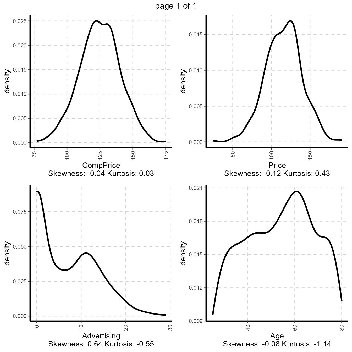

3.1.3. Summary of categorical variables

frequency for all categorical independent variables

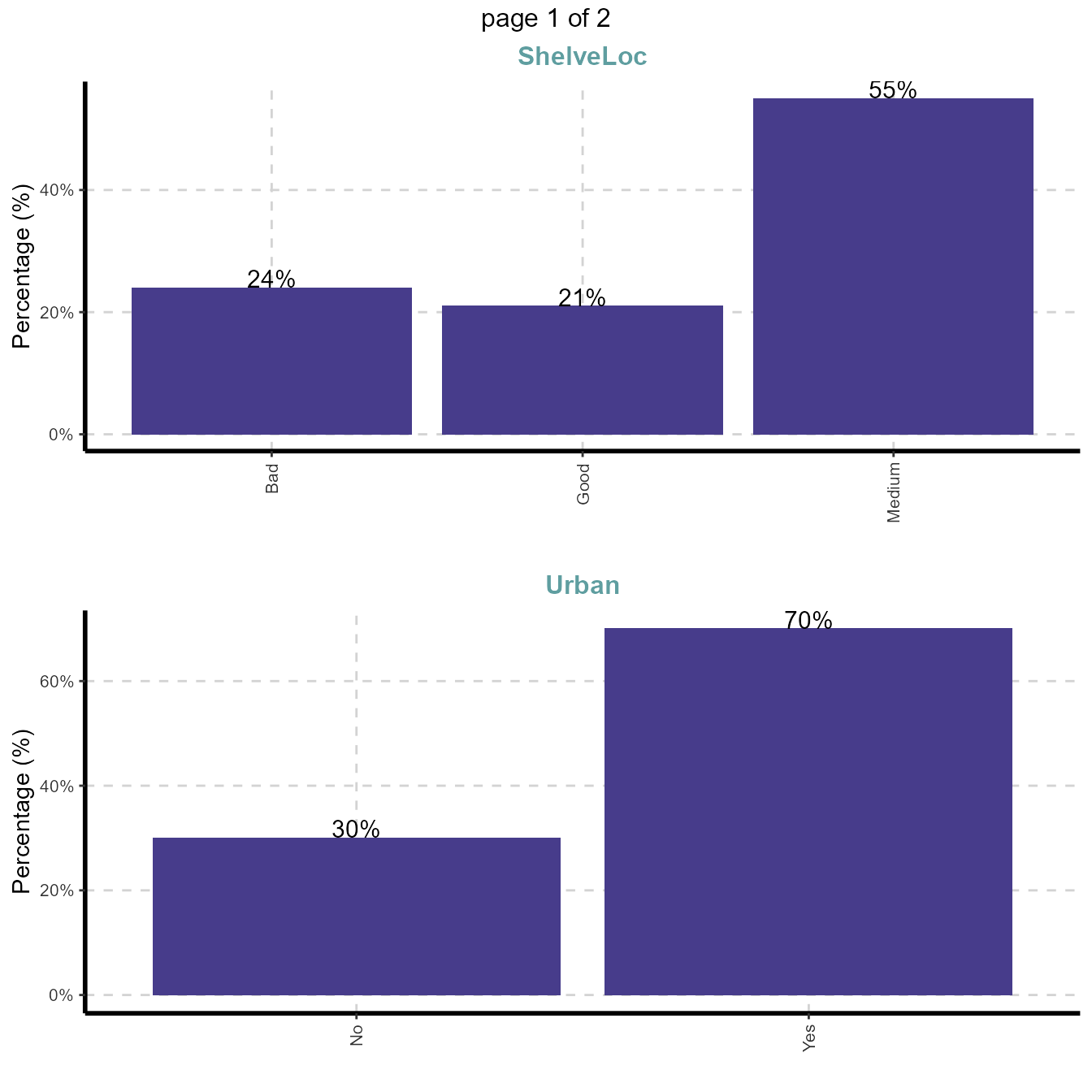
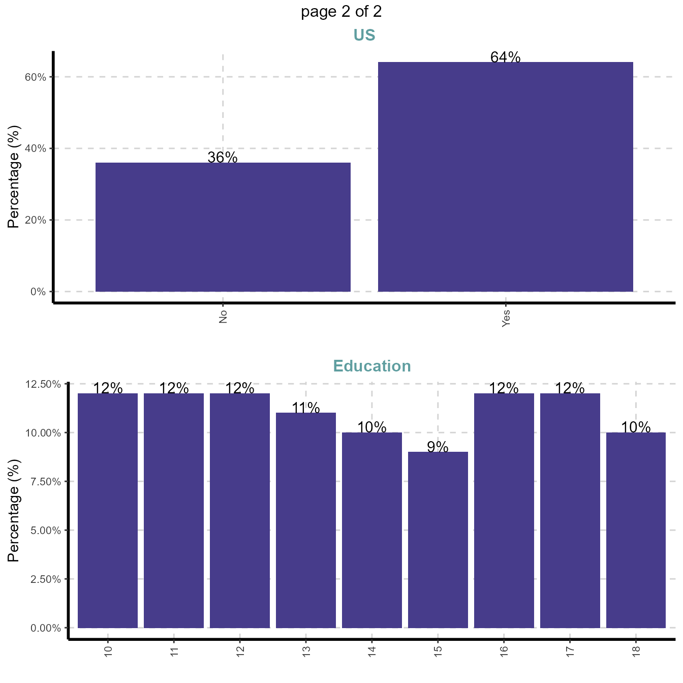
ExpCTable(Carseats,Target=NULL,margin=1,clim=10,nlim=3,round=2,bin=NULL,per=T)

Variable	Valid	Frequency	Percent	CumPercent
ShelveLoc	Bad	96	24.00	24.00
ShelveLoc	Good	85	21.25	45.25
ShelveLoc	Medium	219	54.75	100.00
ShelveLoc	TOTAL	400	NA	NA
Urban	No	118	29.50	29.50
Urban	Yes	282	70.50	100.00
Urban	TOTAL	400	NA	NA
US	No	142	35.50	35.50
US	Yes	258	64.50	100.00
US	TOTAL	400	NA	NA

NA is Not Applicable

3.1.4. Distributions of categorical variables

Bar plots for all categorical variables

plot2 <- ExpCatViz(Carseats,target=NULL,col ="slateblue4",clim=10,margin=2,Page = c(2,1),sample=4)
plot2[[1]]

3.2 Example for case 2: Target variable is continuous

3.2.1. Target variable

Summary of continuous dependent variable

Variable name - Price
Variable description - Price company charges for car seats at each site

summary(Carseats[,"Price"])

##    Min. 1st Qu.  Median    Mean 3rd Qu.    Max. 
##    24.0   100.0   117.0   115.8   131.0   191.0

3.2.2 Summary of numerical variables

Summary statistics when dependent variable is continuous Price.

ExpNumStat(Carseats,by="A",gp="Price",Qnt=seq(0,1,0.1),MesofShape=1,Outlier=TRUE,round=2)

If Target variable is continuous, summary statistics will add the correlation column (Correlation between Target variable vs all independet variables)

3.2.3 Distributions of numerical variables

Graphical representation of all numeric variables

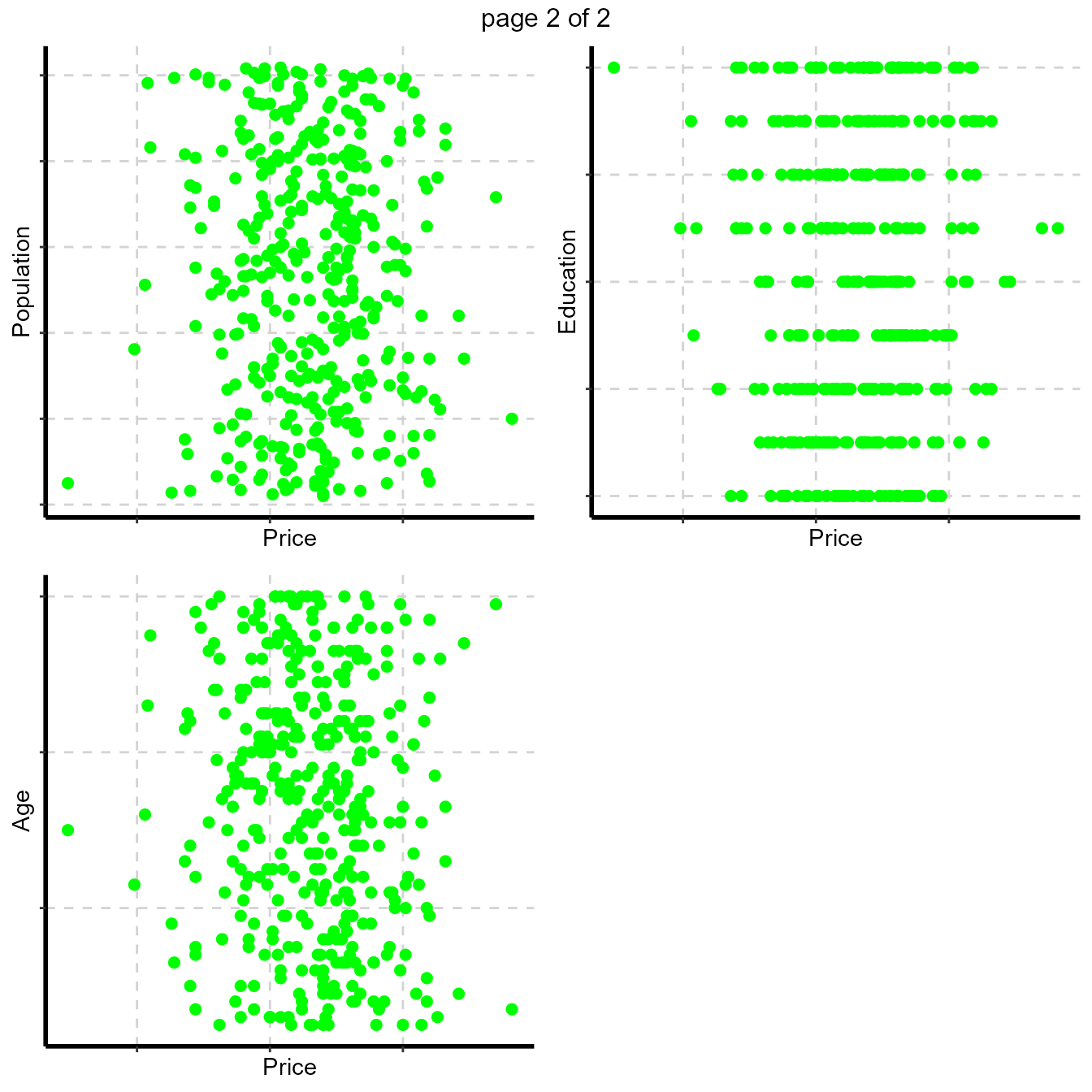
Scatter plot (Bivariate) - with continuous dependent variable

Scatter plot between all numeric variables and target variable Price. This plot help to examine how well a target variable is correlated with dependent variables.

Dependent variable is Price (continuous).

#Note: sample=8 means randomly selected 8 scatter plots
#Note: nlim=4 means included numeric variable with unique value is more than 4
plot3 <- ExpNumViz(Carseats,target="Price",nlim=4,scatter=FALSE,fname=NULL,col="green",Page=c(2,2),sample=8)
plot3[[1]]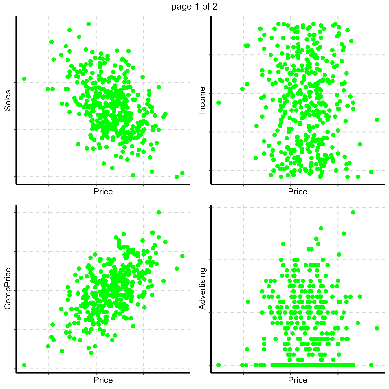

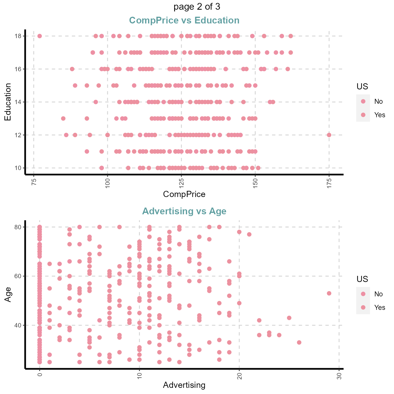
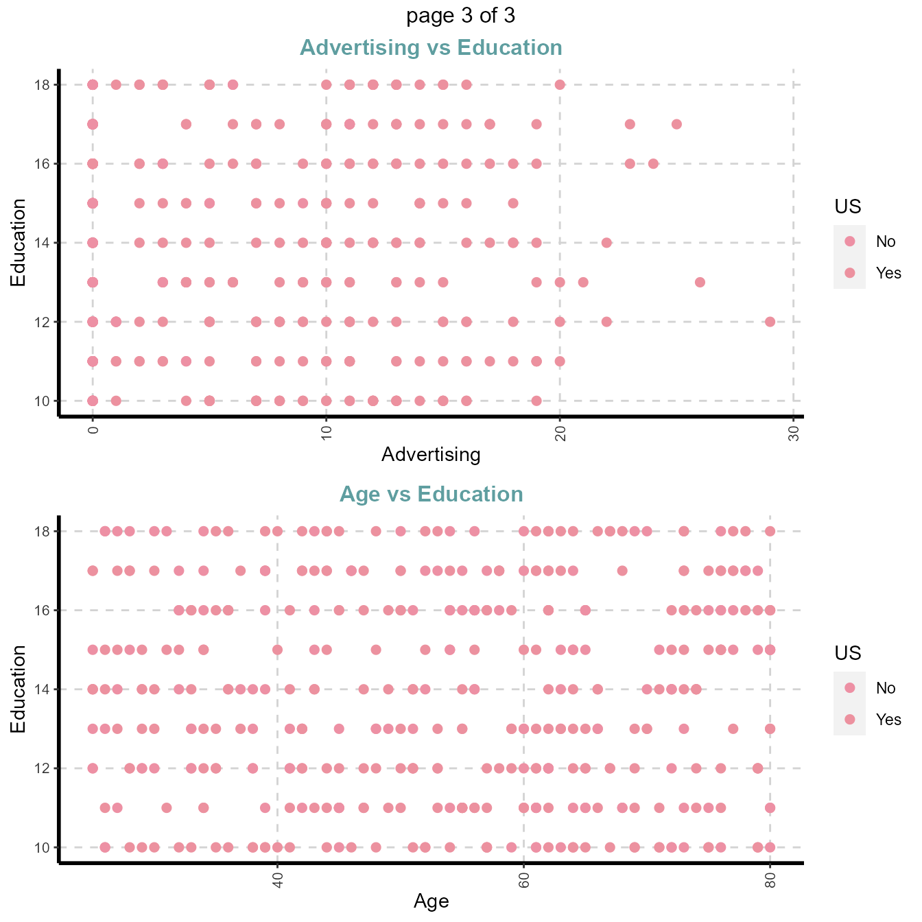
Scatter plot (Bivariate) - between all the numerical variables

#Note: sample=8 means randomly selected 8 scatter plots
#Note: nlim=4 means included numeric variable with unique value is more than 4
plot31 <- ExpNumViz(Carseats,target="US",nlim=4,scatter=TRUE,fname=NULL,Page=c(2,1),sample=4)
plot31[[1]]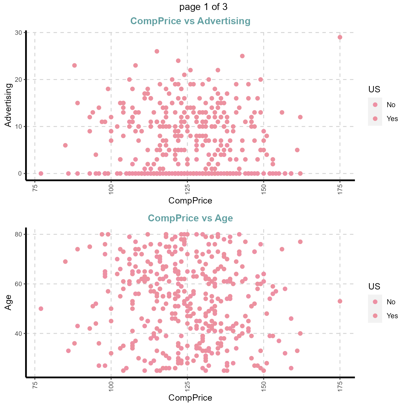

3.2.4. Summary of categorical variables

Summary of categorical variables

frequency for all categorical independent variables by descretized Price

##bin=4, descretized 4 categories based on quantiles
ExpCTable(Carseats,Target="Price",margin=1,clim=10,round=2,bin=4,per=F)

3.3 Example for case 3: Target variable is categorical

3.3.1. Summary of categorical dependent variable

Variable name - Urban
Variable description - Whether the store is in an urban or rural location

Urban	Frequency	Descriptions
No	118	Store location
Yes	282	Store location

3.3.2 Summary of numerical variables

Summary of all numeric variables

ExpNumStat(Carseats,by="GA",gp="Urban",Qnt=seq(0,1,0.1),MesofShape=2,Outlier=TRUE,round=2)

3.3.3 Distributions of Numerical variables

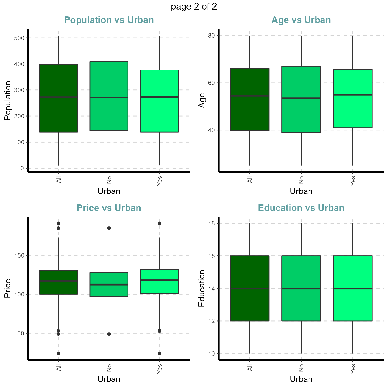
Box plots for all numerical variables vs categorical dependent variable - Bivariate comparision only with categories

Boxplot for all the numeric attributes by each category of Urban

plot4 <- ExpNumViz(Carseats,target="Urban",type=1,nlim=3,fname=NULL,col=c("darkgreen","springgreen3","springgreen1"),Page=c(2,2),sample=8)
plot4[[1]]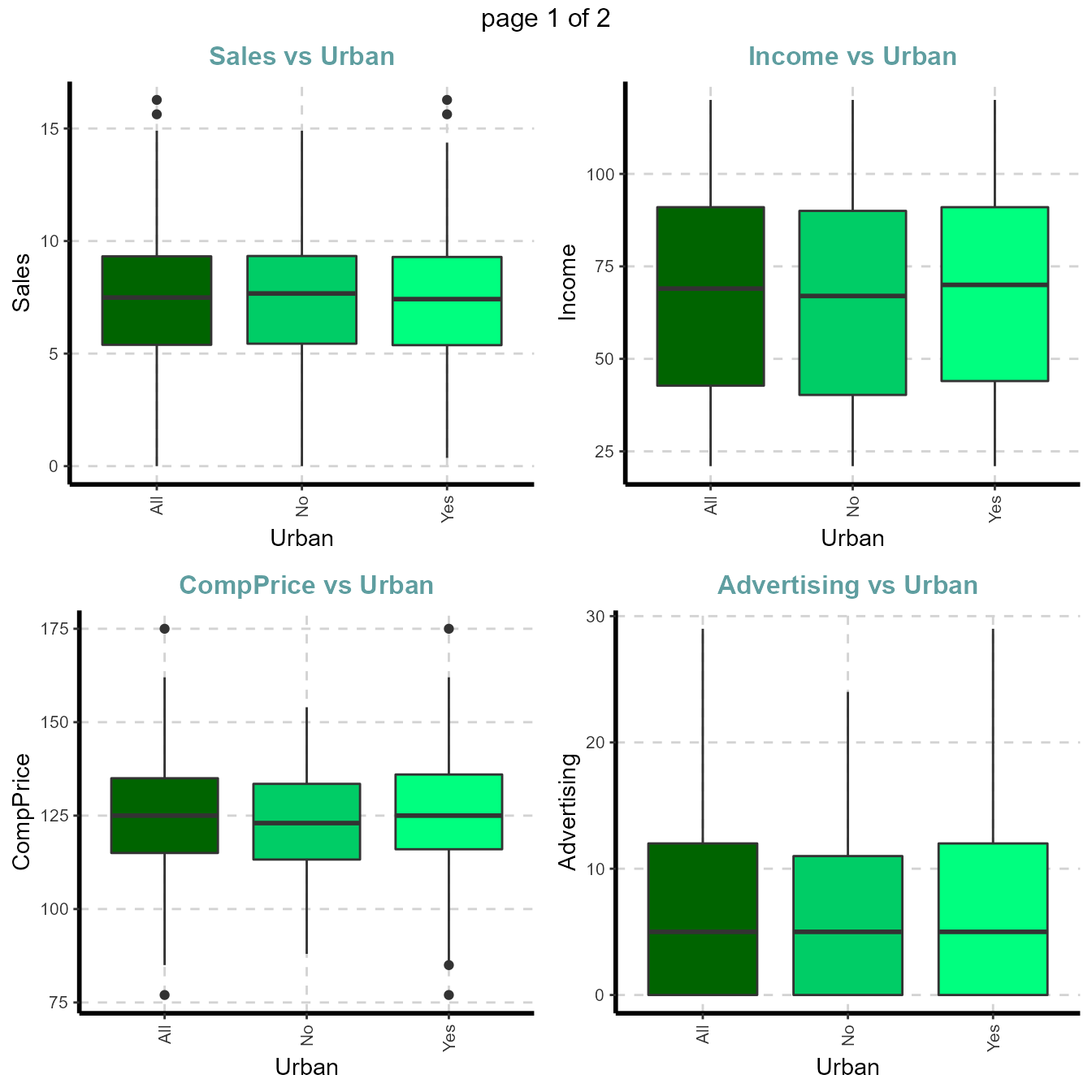

3.3.4 Summary of categorical variables

Cross tabulation with target variable

Custom tables between all categorical independent variables and target variable Urban

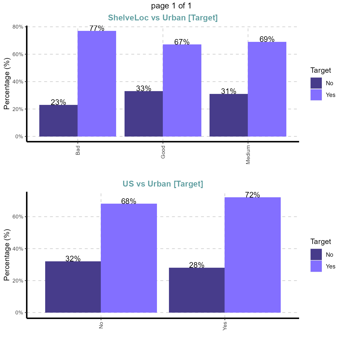
ExpCTable(Carseats,Target="Urban",margin=1,clim=10,nlim=3,round=2,bin=NULL,per=F)

VARIABLE	CATEGORY	Urban:No	Urban:Yes	TOTAL
ShelveLoc	Bad	22	74	96
ShelveLoc	Good	28	57	85
ShelveLoc	Medium	68	151	219
ShelveLoc	TOTAL	118	282	400
US	No	46	96	142
US	Yes	72	186	258
US	TOTAL	118	282	400

Information Value

ExpCatStat(Carseats,Target="Urban",result = "IV",clim=10,nlim=5,bins=10,Pclass="Yes",plot=FALSE,top=20,Round=2)

Variable	Class	Out_1	Out_0	TOTAL	Per_1	Per_0	Odds	WOE	IV	Ref_1	Ref_0	Target
ShelveLoc.1	Bad	74	22	96	0.26	0.19	1.55	0.31	0.02	Yes	No	Urban
ShelveLoc.2	Good	57	28	85	0.20	0.24	0.81	-0.19	0.01	Yes	No	Urban
ShelveLoc.3	Medium	151	68	219	0.54	0.58	0.85	-0.07	0.00	Yes	No	Urban
US.1	No	96	46	142	0.34	0.39	0.81	-0.14	0.01	Yes	No	Urban
US.2	Yes	186	72	258	0.66	0.61	1.24	0.08	0.00	Yes	No	Urban
Sales.1	[0,4.11]	29	11	40	0.10	0.09	1.11	0.10	0.00	Yes	No	Urban
Sales.2	(4.11,5.05]	29	11	40	0.10	0.09	1.11	0.10	0.00	Yes	No	Urban
Sales.3	(5.05,5.86]	26	14	40	0.09	0.12	0.75	-0.29	0.01	Yes	No	Urban
Sales.4	(5.86,6.59]	30	10	40	0.11	0.08	1.29	0.32	0.01	Yes	No	Urban
Sales.5	(6.59,7.49]	32	9	41	0.11	0.08	1.55	0.32	0.01	Yes	No	Urban
Sales.6	(7.49,8.07]	30	9	39	0.11	0.08	1.44	0.32	0.01	Yes	No	Urban
Sales.7	(8.07,8.8]	24	16	40	0.09	0.14	0.59	-0.45	0.02	Yes	No	Urban
Sales.8	(8.8,9.71]	26	14	40	0.09	0.12	0.75	-0.29	0.01	Yes	No	Urban
Sales.9	(9.71,11.28]	26	14	40	0.09	0.12	0.75	-0.29	0.01	Yes	No	Urban
Sales.10	(11.28,16.27]	30	10	40	0.11	0.08	1.29	0.32	0.01	Yes	No	Urban

Statistical test

et4 <- ExpCatStat(Carseats,Target="Urban",result = "Stat",clim=10,nlim=5,bins=10,Pclass="Yes",plot=FALSE,top=20,Round=2)

Variable	Target	Unique	Chi-squared	p-value	df	IV Value	Cramers V	Degree of Association	Predictive Power
ShelveLoc	Urban	3	2.738	0.254	2	0.03	0.08	Very Weak	Not Predictive
US	Urban	2	0.684	0.408	1	0.01	0.04	Very Weak	Not Predictive
Sales	Urban	10	6.696	0.669	9	0.09	0.13	Weak	Somewhat Predictive
CompPrice	Urban	10	4.543	0.872	9	0.03	0.11	Weak	Not Predictive
Income	Urban	10	8.428	0.492	9	0.08	0.15	Weak	Not Predictive
Advertising	Urban	7	5.565	0.474	6	0.06	0.12	Weak	Not Predictive
Population	Urban	10	10.560	0.307	9	0.14	0.16	Weak	Somewhat Predictive
Price	Urban	10	11.143	0.266	9	0.14	0.17	Weak	Somewhat Predictive
Age	Urban	10	8.414	0.493	9	0.08	0.15	Weak	Not Predictive
Education	Urban	8	5.122	0.645	7	0.05	0.11	Weak	Not Predictive

Variable importance based on Information value

varimp <- ExpCatStat(Carseats,Target="Urban",result = "Stat",clim=10,nlim=5,bins=10,Pclass="Yes",plot=TRUE,top=10,Round=2)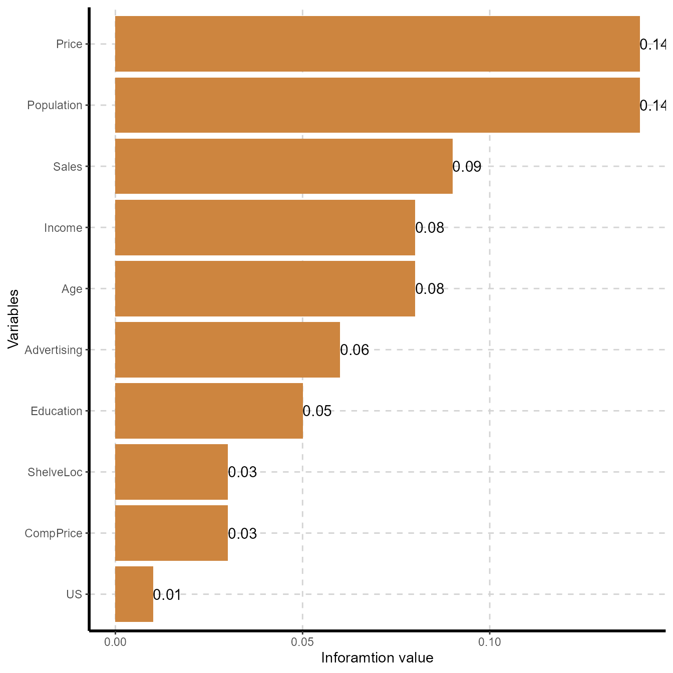

3.3.5. Distributions of categorical variables

Stacked bar plot with vertical or horizontal bars for all categorical variables

plot5 <- ExpCatViz(Carseats,target="Urban",fname=NULL,clim=5,col=c("slateblue4","slateblue1"),margin=2,Page = c(2,1),sample=2)
plot5[[1]]

4. Quantile-quantile plot for numeric variables

Function definition:

ExpOutQQ (data,nlim=3,fname=NULL,Page=NULL,sample=NULL)
data    : Input dataframe or data.table
nlim    : numeric variable limit
fname   : output file name (Output will be in PDF format)
Page    : output pattern. if Page=c(3,2), It will generate 6 plots with 3 rows and 2 columns
sample  : random number of plots

Carseats data from ISLR package:

options(width = 150)
CData = ISLR::Carseats
qqp <- ExpOutQQ(CData,nlim=10,fname=NULL,Page=c(2,2),sample=4)
qqp[[1]]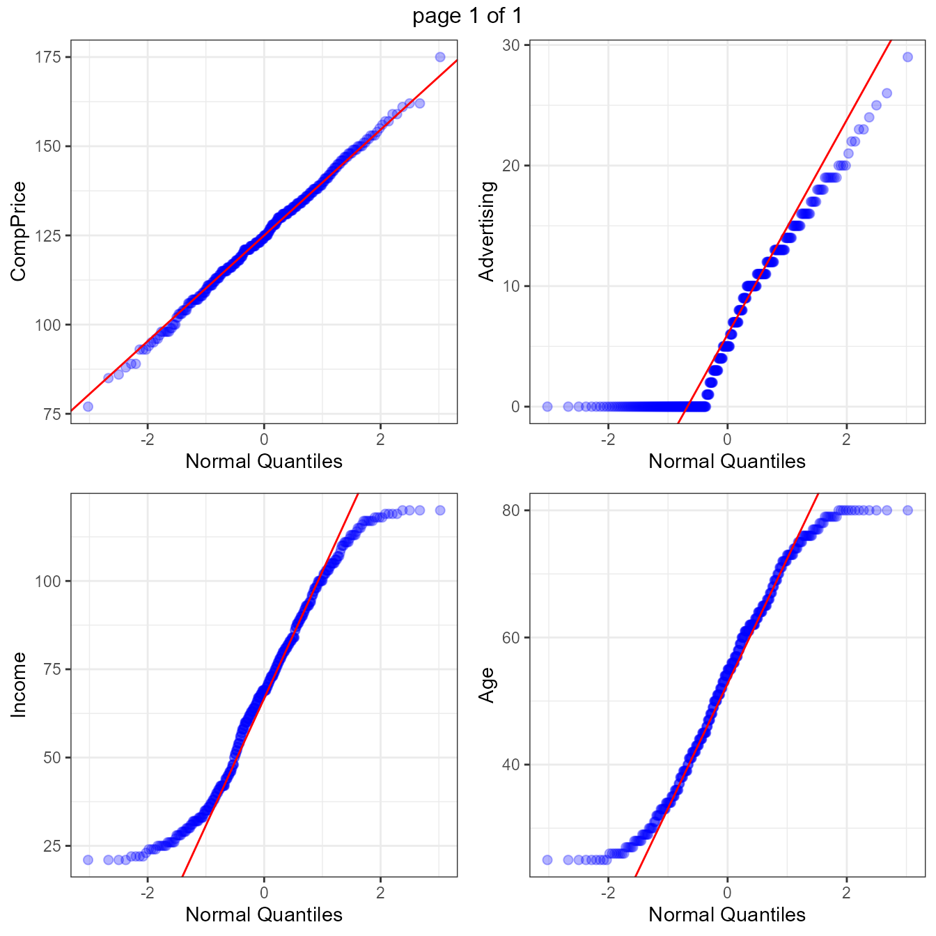

5. Parallel Co-ordinate plots

Function definition:

ExpParcoord (data,Group=NULL,Stsize=NULL,Nvar=NULL,Cvar=NULL,scale=NULL)
data    : Input dataframe or data.table
Group   : stratification variables
Stsize  : vector of startum sample sizes
Nvar    : vector of numerice variables, default it will consider all the numeric variable from data
Cvar    : vector of categorical variables, default it will consider all the categorical variable
scale   : scale the variables in the parallel coordinate plot[Default normailized with minimum of the variable is zero and maximum of the variable is one]

5.1 Defualt ExpParcoord funciton

ExpParcoord(CData,Group=NULL,Stsize=NULL,Nvar=c("Price","Income","Advertising","Population","Age","Education"))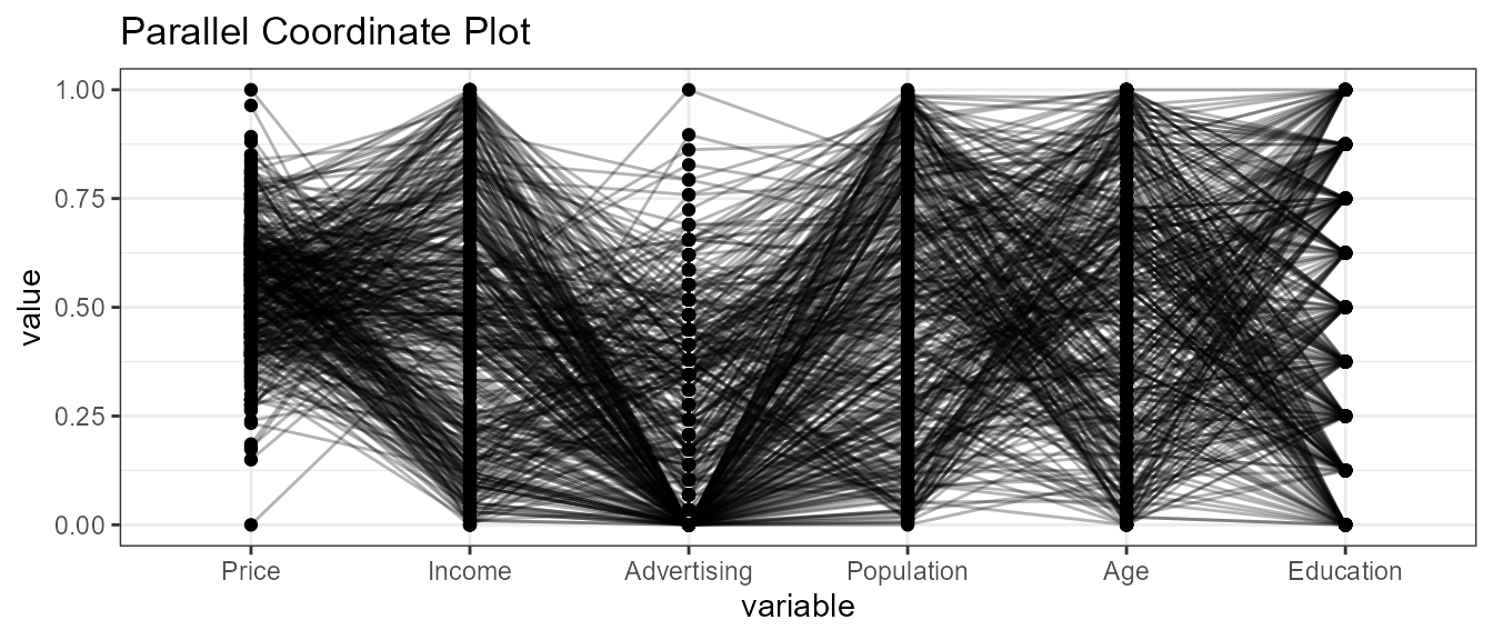

5.2 With Stratified rows and selected columns only

ExpParcoord(CData,Group="ShelveLoc",Stsize=c(10,15,20),Nvar=c("Price","Income"),Cvar=c("Urban","US"))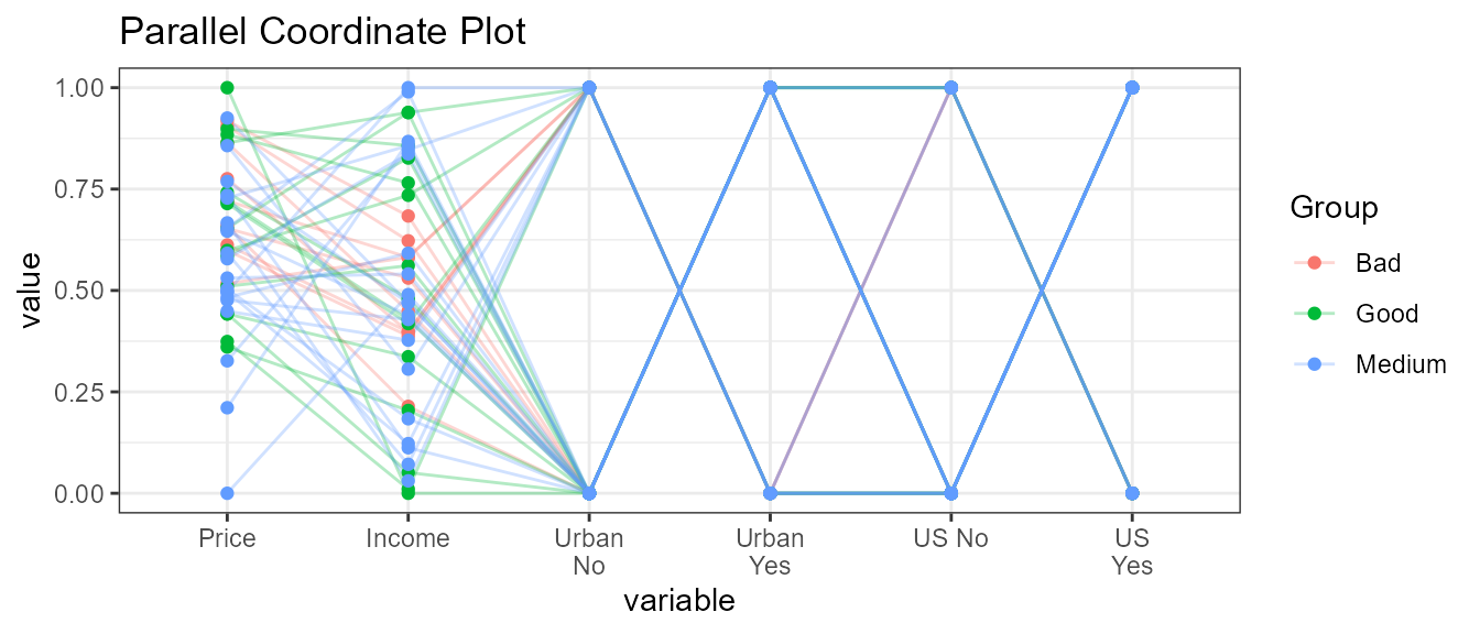

5.3 Without stratification

ExpParcoord(CData,Group="ShelveLoc",Nvar=c("Price","Income"),Cvar=c("Urban","US"),scale=NULL)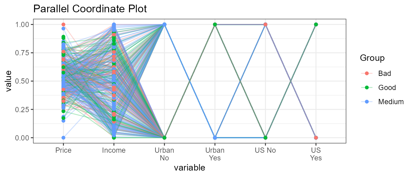

5.4 Scale change

std: univariately, subtract mean and divide by standard deviation

ExpParcoord(CData,Group="US",Nvar=c("Price","Income"),Cvar=c("ShelveLoc"),scale="std")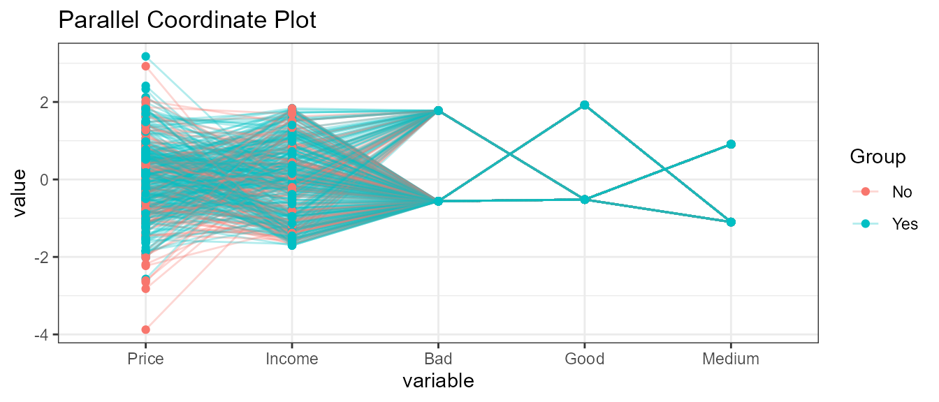

5.5 Selected numeric variables

ExpParcoord(CData,Group="ShelveLoc",Stsize=c(10,15,20),Nvar=c("Price","Income","Advertising","Population","Age","Education"))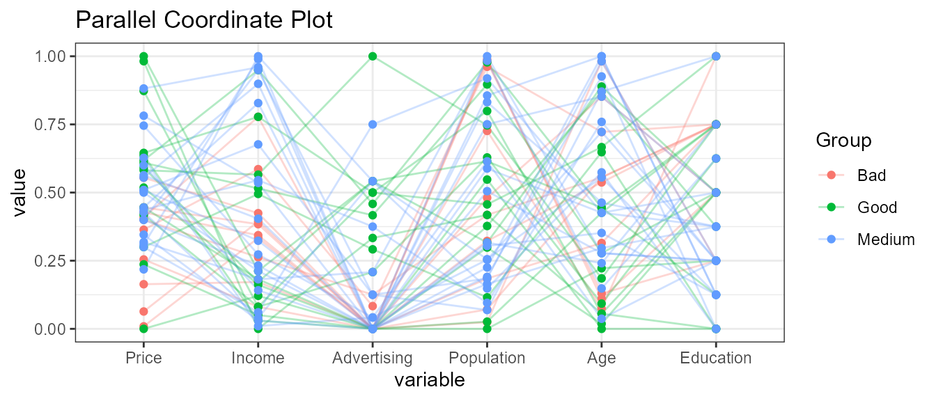

5.6 Selected categorical variables

ExpParcoord(CData,Group="US",Stsize=c(15,50),Cvar=c("ShelveLoc","Urban"))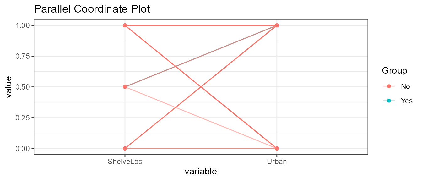

6. Customized Summary Statistics

Used ‘data.table’ package functions

Function definition:

ExpCustomStat(data,Cvar=NULL,Nvar=NULL,stat=NULL,gpby=TRUE,filt=NULL,dcast=FALSE)

ExpCustomStat examples

ExpCustomStat(Carseats,Cvar="Urban",Nvar=c("Age","Price"),stat=c("mean","count"),gpby=TRUE,dcast=F)

Urban	Attribute	mean	count
Yes	Age	53.62057	282
No	Age	52.61017	118
Yes	Price	116.51418	282
No	Price	114.07627	118

ExpCustomStat(Carseats,Cvar="Urban",Nvar=c("Age","Price"),stat=c("mean","count"),gpby=TRUE,dcast=T)

Attribute	mean_No	mean_Yes	count_No	count_Yes
Age	52.61017	53.62057	118	282
Price	114.07627	116.51418	118	282

ExpCustomStat(Carseats,Cvar=c("Urban","ShelveLoc"),Nvar=c("Age","Price","Advertising","Sales"),stat=c("mean"),gpby=FALSE,dcast=T)

Attribute	ShelveLoc_Bad	ShelveLoc_Good	ShelveLoc_Medium	Urban_No	Urban_Yes
Advertising	6.218750	7.352941	6.538813	6.203390	6.815603
Age	52.052083	52.611765	54.155251	52.610169	53.620567
Price	114.270833	117.882353	115.652968	114.076271	116.514184
Sales	5.522917	10.214000	7.306575	7.563559	7.468191

7. Univariate outlier analysis

In statistics, an outlier is a data point that differs significantly from other observations. An outlier may be due to variability in the measurement or it may indicate experimental error; the latter are sometimes excluded from the data set.An outlier can cause serious problems in statistical analyses.

Function ExpOutliers can run univariate outlier analysis based on boxplot or SD method. The function returns the summary of oultlier for selected numeric features and adding new features if there are any outlers

Identifying outliers: There are several methods we can use to identify outliers. In ExpOutliers used two methods (1) Boxplot and (2) Standard Deviation

7.1 Identifying outliers using Boxplot method

ExpOutliers(Carseats, varlist = c("Sales","CompPrice","Income"), method = "boxplot",  treatment = "mean", capping = c(0.1, 0.9))

Summary

Category	Sales	CompPrice	Income
Lower cap : 0.1	4.119	106	30
Upper cap : 0.9	11.3	145	107
Lower bound	-0.5	85	-29.62
Upper bound	15.21	165	163.38
Num of outliers	2	2	0
Lower outlier case		43
Upper outlier case	317,377	311
Mean before	7.5	124.97	68.66
Mean after	7.45	124.97	68.66
Median before	7.49	125	69
Median after	7.47	125	69

Output data head view

Sales	CompPrice	Income	Advertising	Population	Price	ShelveLoc	Age	Education	Urban	US	out_cap_Sales	out_cap_CompPrice	out_imp_Sales	out_imp_CompPrice
9.50	138	73	11	276	120	Bad	42	17	Yes	Yes	9.50	138	9.50	138
11.22	111	48	16	260	83	Good	65	10	Yes	Yes	11.22	111	11.22	111
10.06	113	35	10	269	80	Medium	59	12	Yes	Yes	10.06	113	10.06	113
7.40	117	100	4	466	97	Medium	55	14	Yes	Yes	7.40	117	7.40	117
4.15	141	64	3	340	128	Bad	38	13	Yes	No	4.15	141	4.15	141
10.81	124	113	13	501	72	Bad	78	16	No	Yes	10.81	124	10.81	124

7.2 Identifying outliers using 3 Standard Deviation method

ExpOutliers(Carseats, varlist = c("Sales","CompPrice","Income"), method = "3xStDev",  treatment = "medain", capping = c(0.1, 0.9))

Summary

Category	Sales	CompPrice	Income
Lower cap : 0.1	4.119	106	30
Upper cap : 0.9	11.3	145	107
Lower bound	-0.98	78.97	-15.3
Upper bound	15.97	170.98	152.62
Num of outliers	1	2	0
Lower outlier case		43
Upper outlier case	377	311
Mean before	7.5	124.97	68.66
Mean after	7.47	124.97	68.66
Median before	7.49	125	69
Median after	7.49	125	69

Output data head view

Sales	CompPrice	Income	Advertising	Population	Price	ShelveLoc	Age	Education	Urban	US	out_cap_Sales	out_cap_CompPrice	out_imp_Sales	out_imp_CompPrice
9.50	138	73	11	276	120	Bad	42	17	Yes	Yes	9.50	138	9.50	138
11.22	111	48	16	260	83	Good	65	10	Yes	Yes	11.22	111	11.22	111
10.06	113	35	10	269	80	Medium	59	12	Yes	Yes	10.06	113	10.06	113
7.40	117	100	4	466	97	Medium	55	14	Yes	Yes	7.40	117	7.40	117
4.15	141	64	3	340	128	Bad	38	13	Yes	No	4.15	141	4.15	141
10.81	124	113	13	501	72	Bad	78	16	No	Yes	10.81	124	10.81	124

R package that automates most of exploratory analyses tasks in modeling

Dayananda Ubrangala, Kiran R, Ravi Prasad Kondapalli, Sayan Putatunda

2021-04-03

1. Introduction

Journal of Open Source Software Article

2. Data

2.1 Overview of the data

2.2 Add summary statistics into Metadata ouput

3. Exploratory data analysis (EDA)

3.1 Example for case 1: Target variable is not defined

3.1.1 Summary of numerical variables

3.1.2 Distributions of numerical variables

3.1.3. Summary of categorical variables

3.1.4. Distributions of categorical variables

3.2 Example for case 2: Target variable is continuous

3.2.1. Target variable

3.2.2 Summary of numerical variables

3.2.3 Distributions of numerical variables

3.2.4. Summary of categorical variables

3.3 Example for case 3: Target variable is categorical

3.3.1. Summary of categorical dependent variable

3.3.2 Summary of numerical variables

3.3.3 Distributions of Numerical variables

3.3.4 Summary of categorical variables

3.3.5. Distributions of categorical variables

4. Quantile-quantile plot for numeric variables

5. Parallel Co-ordinate plots

5.1 Defualt ExpParcoord funciton

5.2 With Stratified rows and selected columns only

5.3 Without stratification

5.4 Scale change

5.5 Selected numeric variables

5.6 Selected categorical variables

6. Customized Summary Statistics

7. Univariate outlier analysis

7.1 Identifying outliers using Boxplot method

7.2 Identifying outliers using 3 Standard Deviation method